The first time I ran a circuit on real quantum hardware after it behaved perfectly in simulation, the output made no sense. The distribution did not resemble the theoretical prediction, and repeating the run only made the mismatch more obvious. In classical debugging, this would have been trivial to isolate with print statements or breakpoints. In quantum computing, inspection itself alters the computation. Measurement collapses the state, and even small changes in circuit structure affect the result. On top of that, the device contributes its own behavior: calibration drift, readout bias, crosstalk between qubits, and gate imperfections that never appear in an ideal simulator. [1]
[2]
[3]
In 2026, much of the difficulty in quantum programming lies in validation rather than invention. Developers must determine whether a result reflects the logic of the circuit or the behavior of the hardware. Gate error rates remain significant, queue times discourage repeated experimentation, and calibration changes can invalidate conclusions drawn only hours earlier. It is common to spend substantial time investigating what appears to be a programming error, only to discover that the effect disappears after the next device recalibration.
In practice, the phrase “debugging quantum code” often covers several distinct problems. Some failures originate from incorrect circuit logic. Others arise from compilation and qubit mapping decisions. Many are caused by physical noise that cannot be removed but can be estimated and mitigated. Productive debugging depends on separating these categories instead of treating every anomaly as a single type of bug. The strategies discussed below are built around this separation, reflecting how current tools and workflows have evolved: improved simulators, standardized mitigation techniques, and runtime systems designed for iterative experimentation rather than direct inspection.[4]
[5]
Why Quantum Debugging Still Feels Alien (and Why That’s Not Your Fault)
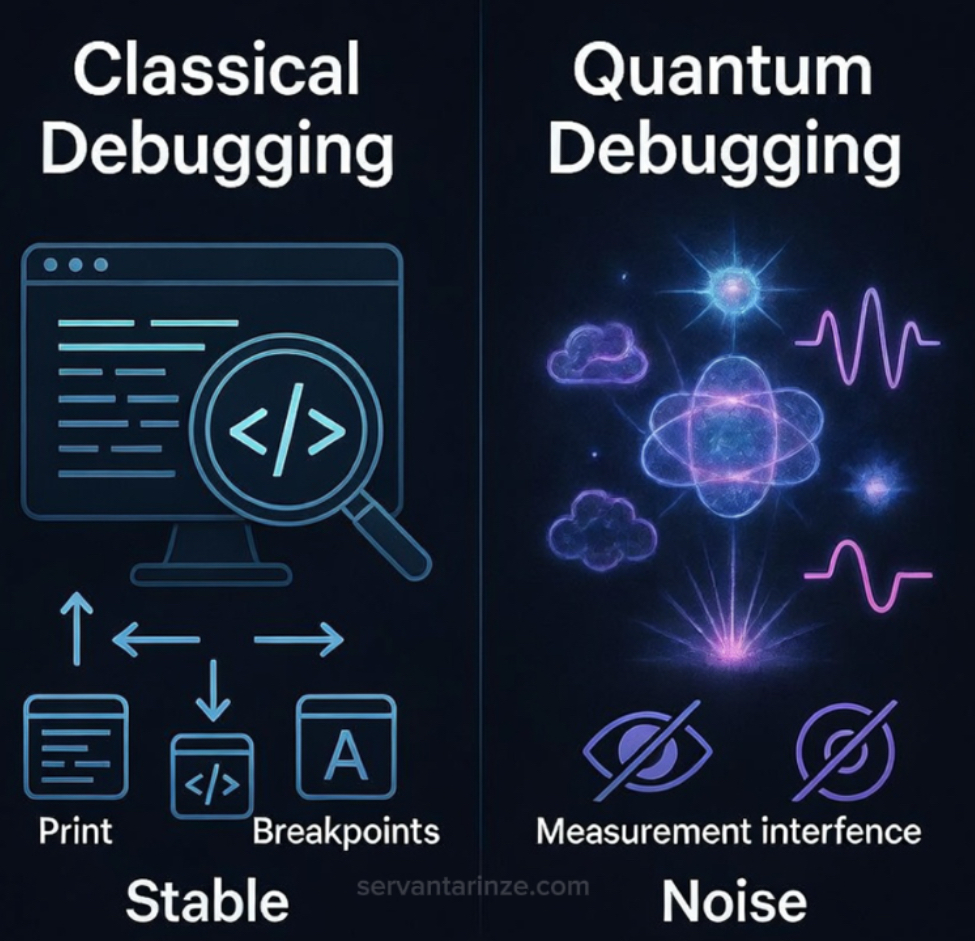
Quantum programs do not fail in the same way as classical programs. Classical bugs usually appear as deterministic errors: a crash, an incorrect value, or a reproducible mismatch. Quantum circuits produce probabilistic outcomes. A single execution is not informative, and even hundreds of shots can be misleading if expectations are poorly defined. Debugging therefore requires analyzing distributions rather than individual results and treating uncertainty as information.
The primary structural limitation is that quantum states cannot be directly inspected without altering them. Measurement collapses the state and changes the computation itself. Indirect methods such as tomography, parity checks, and ancilla-assisted probes provide partial information, but they do not offer the internal visibility available in classical debugging. Debugging therefore relies on inference from limited observations rather than direct inspection.
A second source of difficulty is noise, which arises from multiple mechanisms. Decoherence reduces state fidelity over time. Coherent control errors introduce systematic gate imperfections. Crosstalk allows operations on one qubit to influence neighboring qubits. Readout error alters the final measurement statistics. Because these effects interact, the same circuit can produce different results under different calibration conditions, even when the code remains unchanged.
A further complication arises from compilation and transpilation. The circuit executed on hardware is not the circuit written by the developer. It is mapped to specific qubits, decomposed into native gates, and transformed by optimization passes. These transformations can unintentionally increase circuit depth, alter phase relationships, or route operations through noisy couplings. In many cases, debugging involves identifying whether failure originates from algorithmic logic or from compilation effects.
The objective is therefore not to reproduce classical debugging methods, but to construct workflows that classify the source of error. Effective debugging distinguishes between logical mistakes, compilation artifacts, and physical noise. The methods that follow are designed to support this classification process rather than treating all deviations as undifferentiated failure.
| Classical habit | Quantum reality | Practical substitute |
|---|---|---|
| Print variables | Measurement collapses state | Targeted probes, ancillas, small-system tomography |
| Breakpoints | No step-through visibility | Layer-by-layer circuit slicing + statistical checks |
| Unit tests | Probabilistic outcomes | Assertions over distributions and invariants |
| Reproduce bug reliably | Hardware drift and noise | Simulator comparison + calibration-aware reruns |
Quantum debugging requires more interpretation than classical debugging, but it also becomes systematic with experience. Distributions that initially appear meaningless can be analyzed to determine whether deviations arise from logical structure, device noise, or compilation choices. This shift from reaction to diagnosis marks the transition from trial-and-error to controlled debugging.
The Five Strategies I Trust When Results Go Sideways
1) Simulate Like You Mean It (Ideal vs Noisy vs Hardware)
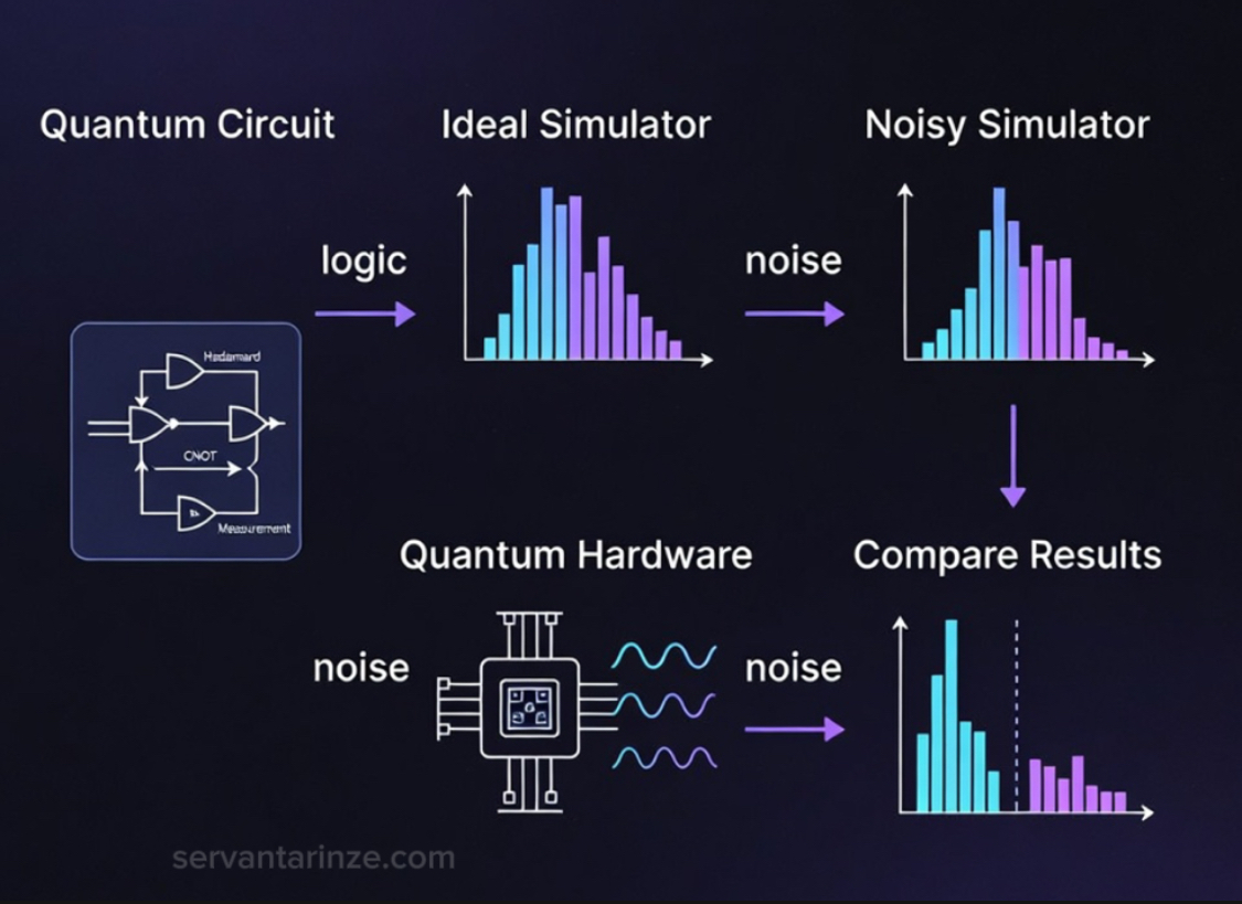
The quickest way to waste time is to send an unverified circuit straight to hardware and then stare at the output as if it’s a confession. Hardware output is evidence that must be interpreted rather than a direct statement of correctness. The cleaner approach is a three-way comparison: ideal simulation, noisy simulation, and hardware execution. If you do this consistently, you catch most logic errors before the queue ever enters the story, and you develop an instinct for what “noise-shaped” results look like.
Ideal simulation tells you what the circuit does in a world without decoherence and readout error. Noisy simulation tells you what the circuit does under a noise model that approximates real devices: depolarizing channels, amplitude damping, measurement flips, and so on. Hardware tells you what happened under the day’s calibration. The classification is often blunt: if ideal and noisy match your expectation but hardware doesn’t, you’re looking at device behavior or mapping choices. If ideal doesn’t match your expectation, you have a logic bug. If ideal matches but noisy doesn’t, you may have built something that is too fragile to survive on NISQ hardware without mitigation.
In Qiskit, that workflow usually means: build the circuit, simulate with a statevector or qasm backend, then simulate again with a noise model derived from a backend’s properties, then run on the backend. In Cirq, the analogous pattern is ideal simulation vs density-matrix simulation (to represent mixed states and noise) vs a hardware sampler.
# Example skeleton (Qiskit-style) for comparing ideal vs noisy vs hardware
from qiskit import QuantumCircuit
from qiskit_aer import Aer
from qiskit_aer.noise import NoiseModel
from qiskit.visualization import plot_histogram

qc = QuantumCircuit(2, 2)
qc.h(0)
qc.cx(0, 1)
qc.measure([0, 1], [0, 1])

# 1) Ideal simulation
ideal_backend = Aer.get_backend("aer_simulator")
ideal_result = ideal_backend.run(qc, shots=4000).result()
ideal_counts = ideal_result.get_counts()

# 2) Noisy simulation (placeholder noise model; in practice build from backend properties)
noise_model = NoiseModel()  # replace with a calibrated noise model when available
noisy_backend = Aer.get_backend("aer_simulator")
noisy_result = noisy_backend.run(qc, shots=4000, noise_model=noise_model).result()
noisy_counts = noisy_result.get_counts()

# 3) Hardware run would go here (via provider backend), then compare counts:
# hardware_counts = ...

# plot_histogram([ideal_counts, noisy_counts, hardware_counts], legend=["ideal", "noisy", "hardware"])
I’ve seen people dismiss noisy simulation because “models aren’t perfect.” That’s true, and it misses the point. The job of noisy simulation isn’t prophecy. It’s triage. It tells you whether your circuit is logically sane and whether it is structurally brittle. Even an imperfect noise model will still highlight obvious fragility: too much depth, interference patterns that evaporate under small decoherence, circuits whose success depends on pristine phases that the device cannot preserve. And when ideal simulation already disagrees with your expectation, you don’t need better hardware—you need better reasoning.
There’s also a quieter benefit: if you store the three distributions (ideal/noisy/hardware) over time, you start noticing patterns. Certain devices bias certain outcomes. Certain qubit pairs behave like trouble. Certain transpilation options quietly change what “works.” That becomes part of your debugging memory.
2) Use Assertions That Respect Quantum Reality (and Still Catch Real Bugs)
Quantum assertions sound like a contradiction until you redefine what “assert” means. In classical code, an assertion checks an exact value at a specific point. In quantum work, you rarely get that luxury. What you can check are invariants and statistical expectations: distributions that should cluster around a known shape, correlations that should appear if entanglement is present, parity relationships that should hold if the circuit is wired correctly, or sanity checks on conserved quantities in small subroutines.
The simplest assertion is a distribution-level test. If you claim you’re generating a Bell state, you don’t need full tomography to catch a broken entangling gate. You can check whether the outcomes are concentrated in the expected bins, and whether the correlation is strong enough to rule out an accidental mixture. On real hardware you’ll tolerate some leakage. The point is to fail loudly when the circuit is wired incorrectly or the mapping destroyed your intent.
# Distribution-level assertion example (conceptual)
# Expected Bell outcomes: "00" and "11" dominate; "01"/"10" should be low.

def bell_assert(counts, min_corr=0.80):
    total = sum(counts.values())
    p00 = counts.get("00", 0) / total
    p11 = counts.get("11", 0) / total
    corr = p00 + p11
    if corr < min_corr:
        raise AssertionError(f"Bell correlation too low: {corr:.3f}")

# bell_assert(hardware_counts, min_corr=0.70)  # loosen threshold on noisy devices
That kind of check catches obvious wiring bugs, but it won’t catch phase errors. Phase bugs are where many developers get humiliated, because a circuit can look “statistically fine” in computational basis measurement and still be wrong. This is where ancilla-assisted checks and basis changes matter. If your algorithm relies on interference, you often need to test in more than one basis. A practical habit is to create a “debug circuit variant” that inserts basis rotations right before measurement so you can test the interference signature directly.
More advanced assertions use ancillas so you can check properties without fully demolishing the computation, but “non-destructive” is a spectrum on NISQ hardware. You can still do something useful: slice your circuit into segments and assert that intermediate distributions fall within expected ranges, using mid-circuit measurements if the platform supports them. The cost is that you are changing the circuit. The payoff is that you stop debugging blind. I’ve used this approach to pinpoint whether the failure appears right after a particular entangling layer or only after a transpiler introduces an unexpected swap chain.
The important mental move is to stop waiting for exactness. Your assertions should be probabilistic, and you should treat them like tests with tolerances, not truths with absolutes. That doesn’t make them weak. It makes them honest.
3) Error Mitigation Is Not a Luxury in 2026 (It’s a Debugging Tool)
Error mitigation is often described as a way to “improve results.” In practice, I use it first as a diagnostic instrument. It helps answer a more fundamental question: am I fighting noise, or am I fighting my own logic? A circuit that only behaves after mitigation may still be logically correct. A circuit that fails even after mitigation is more likely to contain a structural or conceptual error. That distinction saves enormous time and prevents developers from endlessly rewriting code that was never the real problem. [6]
[7]
Three mitigation families dominate real-world work: measurement error mitigation, zero-noise extrapolation, and probabilistic error cancellation. The third is mathematically elegant but resource-intensive and assumption-heavy, so most developers live between the first two. Measurement mitigation is usually the easiest win because readout bias alone can make a correct circuit appear broken. On multi-qubit systems, correlated readout errors are common, and the final histogram can lie in very convincing ways.
Zero-noise extrapolation (ZNE) becomes useful when a circuit is short enough and the observable is stable enough to tolerate multiple executions. The idea is simple but powerful: execute logically equivalent circuits at increasing noise levels, measure the observable each time, and extrapolate backward to estimate what the value would be with zero noise. If that extrapolated value aligns with simulation, you gain confidence that noise—not logic—is dominating the error. If it does not, the debugging lens shifts back to the circuit itself.
# ZNE concept (illustrative pseudocode)
# 1) Define a circuit and an observable.
# 2) Create folded versions that increase noise but preserve the unitary.
# 3) Run each variant on hardware.
# 4) Extrapolate to the zero-noise limit.

scale_factors = [1, 3, 5]
exp_values = []

for s in scale_factors:
    qc_scaled = fold_gates_preserve_unitary(qc, scale_factor=s)  # conceptual
    result = run_on_hardware(qc_scaled, shots=8000)              # conceptual
    exp_values.append(expectation_from_counts(result))

zne_estimate = extrapolate_to_zero_noise(scale_factors, exp_values)
The real debugging value of ZNE lies in the curve, not the final number. Logic bugs rarely scale smoothly with noise. Noise-dominated distortions often do. When expectation values form a coherent trend as noise increases, you are likely observing physical degradation rather than algorithmic failure. When the curve behaves erratically, you may be seeing compilation instability, mapping artifacts, or violated assumptions inside the mitigation model itself.
Mitigation also reveals when a circuit is simply too fragile for the current hardware regime. In those cases, the correct fix is not to change the algorithm but to shorten depth, reroute entanglement paths, or select different qubits with lower error rates. That decision is part of debugging quantum code, even if no line of Python changes.
There is another uncomfortable but valuable role mitigation plays: it exposes overconfidence. When a simulated expectation value feels “obviously right,” mitigation becomes a reality check. If repeated mitigated runs refuse to converge toward that expectation, then the mental model of the circuit may be wrong. Debugging at this level is not about syntax or gates. It is about correcting assumptions.
Error mitigation does not turn NISQ machines into fault-tolerant devices. It does not remove uncertainty. What it does is separate hardware behavior from programmer intent. In a landscape where both are imperfect, that separation is the closest thing quantum developers currently have to a debugger.
4) Visualization Is Where Bugs Become Visible
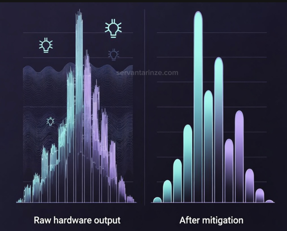
When quantum programs fail, the failure is rarely obvious from raw numbers alone. A table of counts can hide patterns that the human eye would immediately recognize if the same data were drawn as a shape.
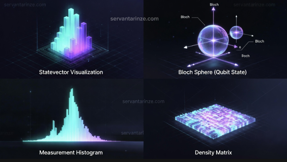
This is why visualization is not cosmetic in quantum development. It is investigative. It is the closest equivalent to stepping through memory states in classical debugging. Histograms, density matrix plots, and statevector reconstructions reveal structure that raw numbers conceal and help identify logical versus physical sources of error. [8]
[9]
I rely on three visual layers: probability histograms, state representations for small circuits, and calibration context. Each reveals a different class of mistakes. Histograms show whether probability mass is leaking into impossible states. State visualizations show phase and coherence errors that simple counts cannot reveal. Calibration overlays explain whether anomalies are physical or logical.
For small circuits, tomography or statevector reconstruction remains the most direct lens. When a Bell state is prepared correctly, its city plot or Bloch representation shows symmetry and phase alignment. When a gate is missing or reversed, that symmetry collapses immediately. No amount of post-processing can hide it. This is how entanglement bugs announce themselves.
from qiskit.visualization import plot_histogram, plot_state_city

# visualize probability distribution
plot_histogram(result.get_counts())

# visualize reconstructed quantum state (small circuits only)
plot_state_city(statevector)
Histograms expose a different class of error: unintended population drift. If probability appears where theory predicts none, the cause is usually one of three things: misordered gates, unwanted basis rotations, or readout bias. Repeating the same circuit with and without transpilation can isolate whether the compiler or the logic introduced the distortion.
Visualization also uncovers temporal instability. When identical circuits executed minutes apart produce visibly different distributions, the bug may not be in the code at all. It may be in calibration drift. Qubits warm. Crosstalk shifts. A debugging session that ignores calibration metadata is blind to half of the problem space.
Phase errors are the most deceptive. Two circuits can share identical measurement histograms while encoding very different quantum states internally. This happens often with interference-based algorithms. Without state inspection or tomography on reduced subsystems, such errors remain invisible. Developers then chase ghosts in logic that is technically correct but physically misaligned.
Visualization also disciplines expectation. When developers imagine what a circuit should “look like,” they build an internal model. Plotting results forces that model to confront reality. Debugging quantum code is often the act of reconciling what one believes the circuit does with what physics permits it to do on imperfect hardware.
Over time, patterns emerge. Certain shapes indicate decoherence. Certain asymmetries point to mapping errors. Certain distortions imply control pulse misalignment. These become part of a developer’s visual vocabulary. Debugging becomes less about individual numbers and more about recognizing signatures.
In classical computing, debugging relies primarily on textual logs and variable inspection. In quantum computing, debugging depends on analyzing distributions, state representations, and geometric patterns in measurement data. Visualization therefore becomes a primary diagnostic method rather than a secondary aid.
5) Iterative Hardware Runs and Calibration-Aware Debugging
Quantum debugging becomes serious only when code leaves the simulator and encounters real hardware . This is where many developers misinterpret noise as logic failure and logic failure as noise. The only way to separate the two is through iterative hardware runs guided by calibration awareness.
I never treat a hardware run as a single verdict. It is one data point in a conversation between code and machine. Each execution must be contextualized by qubit quality, gate fidelities, readout error, and connectivity. A circuit that fails on one backend but succeeds on another is rarely broken in principle. It is broken in placement.
Calibration data exposes the invisible layer of quantum behavior. A qubit with high T1 but poor readout fidelity produces a different error signature than one with low coherence but clean measurement. Without inspecting this metadata, debugging becomes guesswork. The same circuit can appear unstable simply because it was mapped onto an unlucky region of the chip.
Modern runtimes allow developers to lock sessions and reuse calibration windows. This matters because debugging across changing hardware conditions produces contradictory results. A test executed under one calibration set and re-run hours later under another is not a controlled experiment. Iterative debugging requires temporal consistency.
Scaling must be incremental. A circuit that works on two qubits but fails on eight is not evidence of conceptual error. It is evidence of compounded noise. The only meaningful growth path is small-to-large: validate the logic at minimal scale, then expand while tracking how error grows. This mirrors early classical computing, where instability rose with transistor count.
Transpilation strategy itself becomes a debugging tool. Running the same circuit with different optimization levels or layout strategies can reveal whether failure is due to routing complexity rather than algorithmic error. When a bug disappears after remapping, the fault is rarely conceptual. It is architectural.
Hybrid debugging closes the loop. Results from hardware must be compared against noisy simulations seeded with real calibration data. When both agree, the issue is likely logic. When they diverge, the issue is physical. This comparison transforms debugging from frustration into diagnosis.
Queue time also teaches discipline. Hardware access is expensive in both time and opportunity. Debugging quantum code is therefore an exercise in preparation. One does not probe blindly. One designs experiments that isolate variables: change one gate, one qubit, one depth parameter at a time.
Over repeated cycles, a circuit stabilizes. Not because noise disappears, but because the developer learns how to work within it. This is the defining trait of quantum debugging in the NISQ era. It is not about eliminating error. It is about understanding where error enters and why.
In this sense, debugging quantum code resembles experimental physics more than software engineering. Hypotheses are formed. Measurements are taken. Models are refined. The code does not simply run or fail. It reveals behavior, and that behavior must be interpreted.
Once this mindset takes hold, debugging stops feeling like obstruction and starts feeling like investigation. Hardware becomes part of the investigative process rather than an obstacle to correctness.
Common Qubit Error Patterns and How They Reveal Themselves
After enough hardware runs, certain failure patterns begin to repeat. These patterns are not random. They carry signatures that distinguish logical mistakes from physical noise. Learning to recognize them is one of the most valuable skills in debugging quantum code.
The most common logical error is incorrect gate ordering. In classical programming, instruction order matters but variables remain inspectable. In quantum circuits, a single misplaced gate can destroy interference patterns entirely. The output may still look probabilistic, but the distribution will drift far from theoretical expectation even on simulators. This is a strong indicator of conceptual error rather than noise.
Another frequent mistake is unintended disentanglement. Developers often believe two qubits remain entangled when in fact a later gate has broken the correlation. The symptom is subtle: marginal probabilities appear correct, but joint probabilities fail Bell-type checks. This kind of error only becomes visible when correlations are measured explicitly.
Barrier omission also produces misleading behavior. Compiler optimizations can legally reorder gates unless explicitly constrained. A circuit that behaves correctly in theory may be reshaped by transpilation into one that increases depth or introduces fragile interactions. When results fluctuate wildly between optimization levels, this usually points to scheduling rather than algorithmic failure.
Noise-driven errors have their own character. Readout noise produces symmetric distortions around expected peaks. Decoherence produces gradual flattening of distributions. Crosstalk produces unexpected correlations between qubits that should be independent. These patterns are rarely sharp failures. They appear as erosion rather than collapse.
A useful diagnostic is consistency across shots. Logical bugs produce stable wrong answers. Noise produces drifting answers. If thousands of shots cluster around the wrong state, the circuit is wrong. If the distribution spreads unpredictably, the hardware is struggling.
Bell-state preparation failures illustrate this distinction clearly. When entanglement fails because of logic, the simulator and hardware both show incorrect correlations. When it fails because of noise, the simulator remains clean while hardware degrades. The difference between these two cases defines where debugging effort should be focused.
Another pattern involves overconfidence in circuit depth. Developers often underestimate how quickly error compounds. A circuit that performs well at depth 10 may collapse at depth 40. This is not a bug. It is an architectural boundary. Recognizing this prevents wasted time chasing phantom logic errors.
Misinterpreting mitigation as correctness is also dangerous. Error mitigation can make results look right even when logic is flawed. Mitigation should confirm hypotheses, not replace them. A circuit that only works after mitigation is not necessarily correct; it may simply be masked.
One of the most revealing tests is intentional simplification. Remove half the circuit and observe whether behavior stabilizes. If it does, the removed section likely contains the fault. This mirrors classical binary search debugging but operates on circuit topology rather than code lines.
Over time, these patterns build intuition. Debugging quantum code becomes less about fixing syntax and more about interpreting behavior. Each run leaves fingerprints. The task of the developer is to learn how to read them.
When this interpretive skill develops, debugging becomes more structured. Repeated failure patterns can be classified rather than treated as isolated events. Logical faults, compilation artifacts, and physical noise each leave distinguishable signatures in distributions and correlations. Recognizing these signatures allows developers to isolate causes more efficiently and avoid treating hardware variability as algorithmic error.
Tools and Best Practices for Debugging Quantum Code in 2026
The tools available for debugging quantum code in 2026 reflect a field that has accepted its constraints rather than fighting them. There are still no breakpoints. There is still no safe way to inspect a quantum state without destroying it. What has evolved instead is an ecosystem of instruments that treat debugging as statistical diagnosis rather than stepwise inspection.
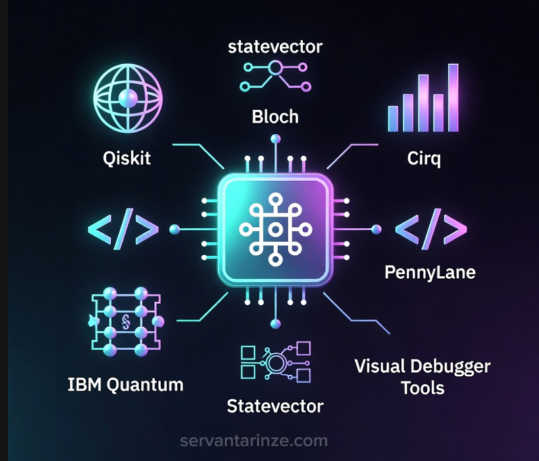
Among programming frameworks, Qiskit remains the most mature environment for structured debugging. Its simulator stack allows side-by-side comparison between ideal statevectors, noisy models, and hardware execution. This layered view has become essential. It mirrors how experimental physicists separate theory, apparatus, and measurement. Cirq and PennyLane follow similar philosophies but differ in emphasis, with Cirq favoring circuit introspection and PennyLane emphasizing hybrid variational workflows.
One noticeable change since the early 2020s is the normalization of calibration-aware development. Developers now routinely consult backend calibration data before choosing qubits or layouts. Debugging no longer begins with code alone. It begins with hardware context. A circuit that fails on one qubit topology may succeed on another without modification.
Visualization tools have become as important as compilers. Histograms, density matrix plots, and fidelity traces reveal structure that raw numbers conceal. When distributions drift, the shape of the drift often reveals the cause. Phase errors appear differently from amplitude decay. Crosstalk leaves asymmetric footprints. These visual signatures are now part of everyday reasoning, not auxiliary diagnostics.
Statistical assertions are emerging as a formal discipline. Instead of checking exact values, developers specify acceptable probability ranges for expected outcomes. A Bell state is not tested for perfection but for correlation above a threshold. A variational circuit is not verified by one result but by convergence behavior over many shots. Debugging becomes probabilistic contract checking rather than deterministic proof.
Version control has also taken on new meaning. Circuits are now tracked not only by code but by hardware configuration and noise model. A working circuit on one backend is not assumed to work on another. This practice has reduced confusion and preserved reproducibility across time.
Best practice increasingly favors small-scale experimentation. Circuits are tested at two or three qubits before being scaled. This is not merely for convenience. It exposes structural bugs that noise would otherwise obscure. The discipline of shrinking problems has become one of the most reliable debugging techniques in quantum development.
Hybrid debugging workflows now dominate. Classical checks validate logic. Quantum runs validate physics. Neither alone is sufficient. Developers oscillate between simulation and hardware the way experimentalists oscillate between theory and apparatus. This rhythm has replaced the classical notion of debugging as linear correction.
Perhaps the most important best practice is restraint. Quantum hardware remains fragile. Every additional gate increases uncertainty. Debugging in 2026 rewards simplicity, not cleverness. The most robust circuits are often the least ornate.
These practices do not eliminate error. They make error interpretable. They transform debugging from guesswork into an experimental science of code.
Challenges and the Future of Debugging Quantum Code
For all the progress made in debugging quantum code, the field remains constrained by physical limits that no software abstraction can remove. Measurement still collapses state. Noise still accumulates faster than logic can correct it. Debugging remains inseparable from hardware behavior, which means every solution is provisional.
The most stubborn challenge is observability. Classical programmers take for granted the ability to inspect memory and variables at will. Quantum developers work inside an opaque system whose internal dynamics can only be inferred indirectly. Tomography offers partial reconstruction, but its exponential cost restricts it to small circuits. As circuits grow, visibility shrinks.
Shot cost is another bottleneck. Debugging requires repetition, yet access to hardware remains limited and expensive in time. Queue delays and fluctuating calibration states introduce uncertainty that has nothing to do with code quality. A circuit that appears broken today may behave differently tomorrow without modification. This instability complicates diagnosis and slows iteration.
Error mitigation, while powerful, is not error correction. It improves expectation values but does not restore true quantum states. Developers must constantly decide whether a deviation reflects flawed logic or imperfect physics. This ambiguity is unique to quantum programming and has no classical parallel.
Quantum debugging introduces conceptual challenges because program correctness cannot be evaluated through single deterministic outputs. Instead, developers must interpret probability distributions produced under noisy conditions. Many observed deviations reflect the difference between idealized theoretical models and imperfect physical implementations rather than coding errors. This places quantum debugging closer to experimental validation than to traditional software testing.
Yet the trajectory is clear. Hardware improvements are already reshaping what debugging looks like. Logical qubits with reduced error rates are beginning to appear in laboratory systems. As coherence times increase, circuits become more interpretable. As error correction matures, debugging will gradually shift from mitigation toward verification.
Machine learning is entering the debugging loop as well. Decoders that infer likely error patterns from measurement data are becoming part of standard toolchains. These systems do not replace reasoning; they augment it, offering statistical insight where human intuition fails.
Future development environments will likely integrate calibration data, assertions, mitigation, and visualization into a single continuous workflow. Debugging will become less about fixing lines of code and more about managing uncertainty across layers of abstraction.
Quantum debugging will continue to resemble experimental workflows in which hypotheses are evaluated through repeated measurement and statistical analysis. Circuit behavior must be validated empirically under specific hardware conditions. This methodology reflects the dependence of quantum software on physical implementation rather than abstract execution alone.
This characteristic reflects the probabilistic nature of quantum computation. Because outcomes must be interpreted statistically rather than deterministically, debugging requires experimental validation rather than direct inspection. This distinguishes quantum software development from classical programming practice.
As quantum processors move beyond the NISQ era, the balance will slowly shift. Errors will become rarer. Logic will dominate noise. But the habits formed now — simulation, mitigation, visualization, statistical reasoning — will persist as the grammar of quantum software development.
The future of debugging quantum code will emphasize improved inference, tighter integration of hardware data, and more systematic validation methods. As hardware reliability increases, debugging will gradually shift from mitigation toward verification of logical correctness.
Conclusion
Debugging quantum code has never been about finding a single wrong line and fixing it. It is a discipline shaped by uncertainty, by physical limits, and by the constant tension between theory and hardware. What looks like a software mistake often turns out to be a property of noise. What appears as noise sometimes reveals a deeper logical flaw.
The developers who succeed in this environment are not those who seek perfect control, but those who learn to work inside probability. They compare simulators to hardware. They assert expectations instead of inspecting variables. They mitigate errors instead of denying them. They visualize distributions rather than chase single outcomes.
Quantum programming in 2026 is still experimental by nature. Every circuit run is a small physics experiment. Every debugging session is an exercise in interpretation. This makes progress slower than in classical software, but it also makes it more honest. The machine does not hide its uncertainty. It exposes it.
The five strategies explored here do not eliminate errors. They make errors legible. They turn confusion into structure and frustration into evidence. That shift is what allows real work to continue despite noisy qubits and imperfect devices.
As hardware improves, some of today’s techniques will fade. Error correction will replace mitigation. Logical qubits will replace fragile physical ones. But the habits formed now — simulation, statistical reasoning, visualization, iteration — will remain the foundation of quantum software practice.
Effective quantum debugging depends less on individual tools than on disciplined interpretation of results. Developers must distinguish between algorithmic intent and physical behavior using simulation, mitigation, and repeated experimentation. This distinction defines the boundary between logical correctness and hardware-induced variation.
The most important lesson is simple: quantum code does not fail silently. It fails probabilistically. Learning to read those probabilities is what turns a quantum programmer into a quantum engineer.
Debugging quantum code represents an early framework for understanding how algorithms interact with physical quantum systems. The practices developed during the NISQ era will inform future approaches to verification and validation as hardware reliability improves.
References
- Nielsen, M. A., & Chuang, I. L. (2010). Quantum Computation and Quantum Information. Cambridge University Press.
https://doi.org/10.1017/CBO9780511976667 - IBM Quantum Documentation – Noise in quantum systems.
https://qiskit.org/documentation/tutorials/noise.html - Preskill, J. (2018). Quantum Computing in the NISQ era and beyond.
https://arxiv.org/abs/1801.00862 - Qiskit Aer Noise Model Documentation.
https://qiskit.org/documentation/apidoc/aer_noise.html - Murali et al. (2019). Noise-Adaptive Compiler Mappings for Noisy Intermediate-Scale Quantum Computers.
https://arxiv.org/abs/1901.11054 - Temme et al. (2017). Error mitigation for short-depth quantum circuits.
https://arxiv.org/abs/1612.02058 - Endo et al. (2021). Hybrid quantum-classical algorithms and error mitigation.
https://arxiv.org/abs/2012.09840 - Qiskit Visualization Tools.
https://qiskit.org/documentation/tutorials/circuits/3_visualization.html - Greenbaum, D. (2015). Introduction to Quantum Gate Set Tomography.
https://arxiv.org/abs/1509.02921
Frequently Asked Questions About Debugging Quantum Code (FAQ)
Why is debugging quantum code harder than classical debugging?
Quantum code cannot be inspected step by step because measurement collapses the quantum state. Instead of reading variables directly, developers must infer correctness from probability distributions, repeated runs, and comparisons with simulation. Noise and decoherence further blur the line between logical bugs and hardware imperfections.
How can I tell whether an error comes from my code or from quantum hardware noise?
The most reliable method is to compare results from an ideal simulator, a noisy simulator, and real hardware. If the simulator behaves as expected but hardware does not, noise is likely responsible. If both disagree with theory, the issue is usually in the circuit logic itself.
Can quantum programs be debugged without running them on real hardware?
Yes, but only partially. Simulation is essential for detecting logical flaws and verifying expected probability distributions. However, real hardware introduces effects such as crosstalk and calibration drift that simulators cannot fully capture. Effective debugging requires both environments.
What role does error mitigation play in debugging quantum code?
Error mitigation does not fix the circuit but clarifies its behavior by reducing the impact of noise on measured results. Techniques such as readout correction and zero-noise extrapolation help distinguish whether unexpected outputs arise from faulty logic or from physical errors in the device.
Are there quantum equivalents of breakpoints and print statements?
Not in the classical sense. Instead of inspecting values directly, quantum developers use assertions, ancilla-based checks, tomography, and statistical tests to verify that a circuit behaves as intended without destroying the computation.
Will fault-tolerant quantum computers eliminate the need for debugging?
No. Fault tolerance will reduce hardware noise but will not remove logical mistakes or design flaws. Debugging will shift from managing physical qubit errors toward validating higher-level quantum algorithms and logical operations.