Mastering OpenQASM 3.0: 7 Advanced Techniques for Quantum Circuit Design

Estimated Reading Time: 21 minutes

Quantum programming has undergone a noticeable shift over the past few years. Early workflows largely treated quantum circuits as static sequences of gates and measurements that were compiled once and then executed on hardware. While this model was sufficient for early demonstrations, it does not fully capture how modern quantum processors behave in practice. Qubits decohere unpredictably, calibration parameters drift, and many practical algorithms require decisions to be made during execution rather than before it begins.¹

That shift is precisely where OpenQASM 3.0 enters the picture. Earlier versions of the language were designed primarily as a straightforward assembly representation for quantum circuits. OpenQASM 2.0 played an important role in standardizing how circuits could be exchanged between tools like Qiskit and various simulators. Yet its model remained largely static: circuits were compiled ahead of execution, classical logic was limited, and timing information was mostly abstracted away from the programmer.²

OpenQASM 3.0 addresses these limitations by extending the original language model. Instead of treating a quantum program as a rigid sequence of instructions, the language now supports dynamic circuits, explicit timing, classical control flow, pulse-level calibration hooks, and parameterized interfaces that integrate naturally with hybrid algorithms. These additions were not theoretical improvements. They emerged directly from the realities of operating modern quantum hardware in the noisy intermediate-scale quantum (NISQ) era.

In practical development environments, a consistent pattern appears: the closer circuit descriptions move toward the hardware abstraction layer, the more control developers gain over performance and stability. High-level frameworks remain essential, but the underlying assembly language determines how those abstractions ultimately translate into real pulses acting on physical qubits. In practice, the difference between a working experiment and a failed one can sometimes be traced back to how precisely a circuit is expressed at this level.

OpenQASM 3.0 therefore represents more than a version upgrade. It is an expansion of the quantum programming model itself. Dynamic circuits enable algorithms to react to measurement outcomes in real time. Timing instructions allow programmers to schedule delays or synchronization points explicitly, opening the door to techniques like dynamical decoupling and crosstalk mitigation. Calibration definitions make it possible to bind high-level gates to hardware-specific pulse implementations without leaving the language environment.

These capabilities are now appearing across several quantum computing platforms. IBM’s quantum systems support dynamic circuits and OpenQASM-compatible workflows through Qiskit, while Amazon Braket integrates OpenQASM execution through its device interfaces and verbatim compilation modes. Other hardware platforms and orchestration systems are gradually aligning with the same direction, reflecting a broader shift toward dynamic quantum circuit execution and hardware-aware programming.³

Many introductory discussions of OpenQASM 3.0 focus primarily on syntax rather than practical circuit design. Documentation often introduces the syntax but stops short of exploring the deeper techniques that make the language powerful in practice. In real research environments, developers rarely write trivial circuits; they construct adaptive routines, calibrate operations, coordinate classical logic, and tune timing behavior to squeeze stability from fragile quantum hardware.

Understanding those deeper techniques is where the real advantage lies. When OpenQASM is used merely as an export format from higher-level frameworks, much of its expressive power remains hidden. But when the language is approached directly—at the level of circuit architecture and hardware behavior—it becomes a remarkably flexible tool for designing sophisticated quantum workflows.

The discussion that follows examines seven advanced techniques that illustrate how OpenQASM 3.0 is used in serious quantum circuit engineering. Each technique reflects capabilities that have become increasingly relevant as researchers push quantum processors toward more complex experiments: dynamic measurement feedback, modifier-based gate composition, explicit timing control, pulse-level calibration definitions, structured classical logic, advanced register handling, and parameterized circuit interfaces for hybrid algorithms.

Taken together, these features shift how quantum programs can be expressed at the assembly level. Instead of thinking of circuits as static diagrams compiled once and executed blindly, OpenQASM 3.0 encourages a model in which circuits behave more like responsive systems—programs capable of interacting with measurement results, adapting execution paths, and aligning closely with the physical timing of the hardware beneath them.

For developers working close to quantum hardware, understanding these capabilities is increasingly important. The difference between a naive circuit and a carefully engineered one can determine whether an experiment produces meaningful data or collapses under noise. Assembly-level awareness does not replace high-level frameworks, but it provides the insight needed to understand how those frameworks ultimately operate.

Studying these techniques provides insight into how modern quantum circuits are executed and controlled, offering a clearer view of how quantum systems are programmed, optimized, and operated in practice.

Working with OpenQASM 3.0 in Practice

Before exploring advanced OpenQASM 3 circuit design, it helps to understand the environment in which these circuits usually live. OpenQASM is rarely used in isolation. In most real-world workflows the language sits between high-level quantum programming frameworks and the physical hardware executing the instructions. Developers often write algorithms in Python-based frameworks such as Qiskit, Cirq, or Braket SDKs, while OpenQASM acts as a lower-level representation describing how the circuit should actually execute.

Because of this role, OpenQASM 3.0 can be approached from two directions. One approach is indirect: write circuits in a high-level framework and export them to OpenQASM. The other approach is direct: design the circuit intentionally at the assembly level, using the language itself to control timing, measurements, and classical logic. The latter method is where the advanced capabilities of the language become most visible.

Most researchers working with OpenQASM 3.0 rely on Python environments that provide access to simulators and hardware backends. Qiskit remains one of the most widely used ecosystems for this purpose, offering tools for constructing circuits, exporting OpenQASM representations, and running experiments on IBM Quantum devices or high-fidelity simulators. Amazon Braket also supports OpenQASM execution models through its device interfaces, particularly when working with hardware providers that expose lower-level circuit descriptions.

A minimal environment typically includes Python, Qiskit, and access credentials for a simulator or quantum device. Once configured, circuits written in Python can be translated into OpenQASM 3 code and executed or inspected directly. This translation layer is important because it reveals how high-level constructs map onto assembly-level instructions.


pip install qiskit


Within Python, a circuit can be generated and exported into OpenQASM representation. The exported code often exposes details that remain hidden when working purely at the framework level. For example, measurement operations, classical registers, and gate definitions become explicit instructions in the OpenQASM program.


from qiskit import QuantumCircuit
from qiskit.qasm3 import dumps

qc = QuantumCircuit(2, 2)
qc.h(0)
qc.cx(0,1)
qc.measure([0,1], [0,1])

print(dumps(qc))


What becomes interesting in OpenQASM 3.0 is that the language no longer behaves as a static export format. It now supports constructs that resemble classical programming languages: conditional logic, loops, timing instructions, and parameterized interfaces. These additions allow the circuit description to respond to events occurring during execution rather than simply executing a predetermined sequence of gates.

That distinction may appear subtle, but it changes how quantum circuits can be designed. Earlier generations of circuits were compiled entirely before execution began. Once the circuit started running, every operation had already been determined. OpenQASM 3.0 introduces the ability for circuits to adapt mid-execution based on measurement outcomes, enabling entirely new algorithmic strategies.

Understanding these dynamic capabilities requires stepping away from the traditional view of circuits as static diagrams. Instead, a circuit becomes something closer to a program interacting with both quantum and classical information streams. Measurement results can influence subsequent operations, classical registers can store intermediate data, and conditional branches can alter the path of execution.

Technique 1: Dynamic Circuits with Classical Feed-Forward

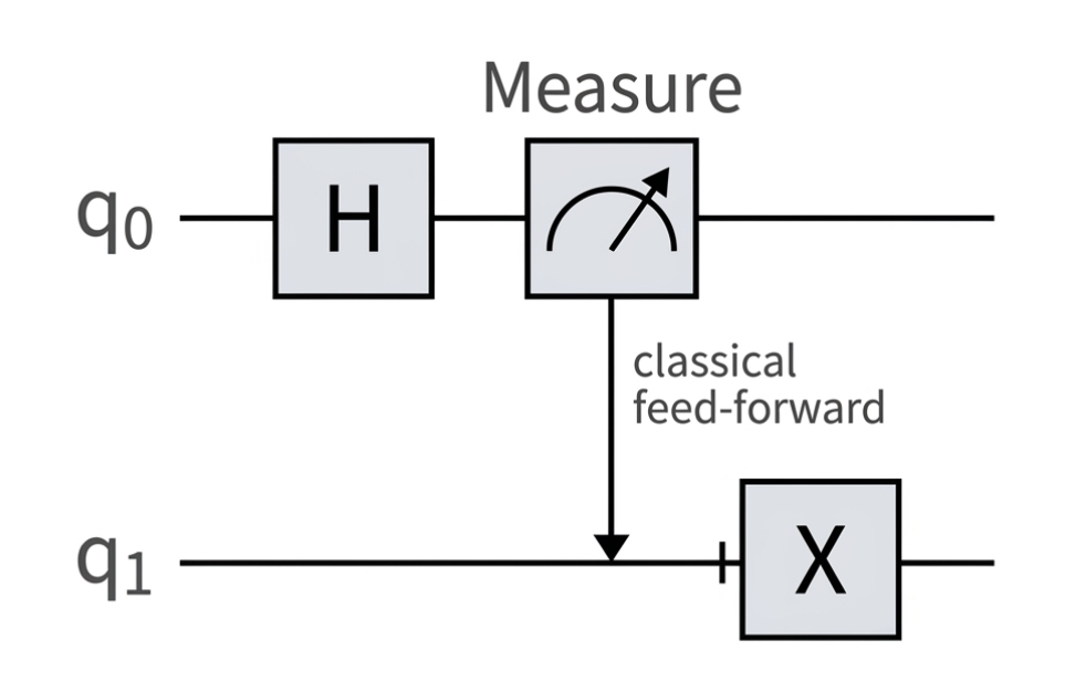
Among the most significant additions to OpenQASM 3.0 is support for dynamic circuits. A dynamic circuit allows measurement results obtained during execution to influence later operations in the same program. In earlier quantum programming models, circuits were compiled in advance and executed without modification. Measurements occurred only at the end of the circuit because there was no mechanism to react to them during runtime.

Modern quantum processors increasingly support mid-circuit measurements and conditional operations. This capability enables circuits to perform adaptive tasks: measuring a qubit, evaluating the outcome using classical logic, and applying subsequent gates depending on the result. The mechanism resembles feedback control systems used in classical engineering, where observations influence the next step in a process.

OpenQASM 3.0 provides syntax for expressing these relationships directly. Classical registers store measurement outcomes, and conditional statements determine which operations follow. The resulting circuits behave less like rigid gate sequences and more like interactive procedures.


OPENQASM 3;

qubit q[2];
bit c[1];

h q[0];
measure q[0] -> c[0];

if (c[0] == 1) {
    x q[1];
}


The program begins by preparing a qubit in superposition. After measurement, the classical result stored in register c determines whether a Pauli-X gate is applied to the second qubit. In practical terms, the circuit reacts to the observed state of the first qubit and modifies the behavior of the second accordingly.

This pattern may appear simple, yet it forms the backbone of many advanced quantum protocols. Teleportation circuits rely on classical feed-forward to reconstruct quantum states. Error correction routines repeatedly measure stabilizers and adjust operations depending on the results. Adaptive phase estimation algorithms refine measurements iteratively based on earlier observations.

From a hardware perspective, implementing dynamic circuits requires tight coordination between the quantum processor and classical control electronics. Measurement outcomes must be processed quickly enough to influence subsequent gate operations without disrupting coherence across the remaining qubits. The improvements in quantum control hardware over the past few years have made this increasingly feasible on real devices.

Because of these hardware constraints, dynamic circuits represent one of the most important frontiers in modern quantum programming. They bridge the gap between quantum computation and classical feedback control, allowing algorithms to interact with measurement results in real time.

Dynamic Circuits in Practice: Adaptive Quantum Behavior

Dynamic circuits become more interesting when the measurement result is not merely toggling a single gate but actively steering the evolution of a larger quantum routine. In laboratory settings, researchers often rely on adaptive behavior to stabilize fragile experiments. Measurements provide information about the system, and the control software reacts immediately, attempting to maintain coherence or correct deviations. OpenQASM 3.0 provides a structured way to express this relationship directly inside the circuit description.

One of the most widely discussed examples is quantum teleportation. The protocol demonstrates how an unknown quantum state can be transferred between two distant qubits using entanglement and classical communication. In a teleportation experiment, measurement outcomes from the sender determine which corrective gates must be applied by the receiver. Without classical feed-forward, the state reconstruction would fail.

OpenQASM allows that behavior to be encoded directly into the program. The circuit measures intermediate qubits, stores the results in classical bits, and conditionally applies correction gates depending on those outcomes. In other words, the quantum program contains both the quantum operations and the classical logic required to complete the protocol.


OPENQASM 3;

qubit q[3];
bit c[2];

h q[1];
cx q[1], q[2];

cx q[0], q[1];
h q[0];

measure q[0] -> c[0];
measure q[1] -> c[1];

if (c[1] == 1) {
    x q[2];
}

if (c[0] == 1) {
    z q[2];
}


In this circuit the first qubit carries the state to be teleported. Qubits one and two share an entangled pair. Measurements on the sender’s side generate classical bits that determine which corrective operations must be applied to the receiver’s qubit. The classical branch instructions represent the feed-forward stage of the teleportation protocol.

From a programming perspective the significance is subtle but important. The circuit does not simply execute a predetermined sequence of operations. It measures the system, evaluates the outcome, and conditionally modifies the remainder of the circuit. This behavior aligns quantum programs more closely with classical control systems used in fields such as robotics or signal processing.

The emergence of dynamic circuits has also influenced hardware architecture. Quantum processors now incorporate classical co-processors designed to process measurement results with minimal latency. These controllers interpret measurement outcomes, evaluate conditional logic, and trigger subsequent gate instructions while the quantum system remains coherent. Without that fast classical processing layer, dynamic circuits would not be practical.

As quantum devices grow in size and complexity, adaptive circuits are expected to become increasingly common. Error mitigation routines, measurement-based algorithms, and certain quantum communication protocols all rely on the ability to incorporate classical feedback within the execution flow. OpenQASM 3.0 provides a language-level mechanism for describing those interactions clearly.

Technique 2: Gate Modifiers for Compact Circuit Design

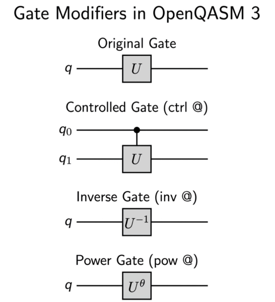
Another powerful feature introduced in OpenQASM 3.0 is the ability to modify gates directly through structured modifiers. Earlier versions of the language required developers to define separate gates for controlled or inverted operations. As circuits became larger, this approach often produced verbose and repetitive code. Gate modifiers offer a more expressive mechanism for constructing complex operations without manually redefining every variant.

The language introduces several modifiers that can transform existing gates. Among the most useful are the inverse modifier, the controlled modifier, and exponentiation through fractional powers. These transformations allow programmers to derive new gate behaviors from existing definitions in a concise and mathematically transparent way.

The inverse modifier is particularly useful in algorithms where operations must be reversed during an uncomputation phase. Many quantum algorithms involve preparing a state, performing intermediate processing, and then applying the inverse of earlier transformations to disentangle auxiliary qubits. Expressing these inverses directly through a modifier simplifies circuit descriptions.


OPENQASM 3;

qubit q[1];

h q[0];
inv @ h q[0];


The statement applies a Hadamard gate followed by its inverse. Since the Hadamard gate is self-inverse, the two operations cancel each other, leaving the qubit unchanged. Although this is a trivial example, the modifier becomes extremely useful when dealing with more complex gates whose inverses would otherwise need to be manually defined.

Controlled modifiers extend this idea further. Instead of defining a controlled version of every gate, OpenQASM allows a programmer to apply a control modifier directly to an existing gate definition. This significantly reduces the complexity of multi-qubit circuits.


OPENQASM 3;

qubit q[2];

ctrl @ x q[0], q[1];


This instruction applies a controlled-X gate, functionally equivalent to the familiar CNOT operation. The advantage becomes clearer when working with more sophisticated gates. A rotation gate or custom operation can be controlled simply by applying the modifier rather than redefining an entirely new gate structure.

Modifiers can also be composed together, allowing multiple transformations to be applied in sequence. For example, a programmer might specify the inverse of a controlled gate or construct multi-controlled operations without explicitly writing them from scratch. These constructs make OpenQASM circuits more expressive while preserving a close relationship with the underlying mathematics of quantum operations.

As quantum processors expand toward larger qubit counts, maintaining readable circuit descriptions becomes increasingly important. Gate modifiers reduce redundancy and encourage modular design, making complex circuits easier to maintain and reason about. They also align naturally with the way many high-level frameworks internally represent operations, creating a smoother transition between abstraction layers.

Extending Gate Modifiers: Powers and Negative Controls

The modifier system in OpenQASM 3.0 extends beyond simple inversion and control. Additional operators allow developers to express fractional powers of gates and conditional operations based on negative control states. These features provide a more flexible language for describing circuit behavior without redefining large numbers of gate variants.

The power modifier allows a gate to be applied repeatedly or fractionally according to an exponent. In mathematical terms, this corresponds to raising the gate’s unitary matrix to a specified power. Fractional powers appear frequently in quantum algorithms where small rotations must be applied repeatedly during iterative procedures.


OPENQASM 3;

qubit q[1];

pow(0.5) @ x q[0];


The instruction above represents the square root of the Pauli-X gate. Such fractional operations often arise in decomposition strategies where a complex unitary must be expressed as a sequence of smaller rotations. In large-scale circuits these compact expressions make the program easier to understand while still mapping directly to the mathematical transformation being applied.

Another useful modifier is the negative control modifier. Classical control logic typically triggers when a control bit equals one. Quantum circuits sometimes require the opposite behavior: executing an operation only when the control qubit is in the zero state. Rather than constructing a workaround using additional gates, OpenQASM allows this logic to be expressed directly.


OPENQASM 3;

qubit q[2];

negctrl @ x q[0], q[1];


In this example the X gate is applied to the second qubit only when the first qubit is in the zero state. Negative controls appear in certain oracle constructions and reversible logic transformations where conditions depend on the absence rather than the presence of a quantum signal.

What makes the modifier system particularly powerful is that multiple modifiers can be composed together. An instruction can be inverted, controlled, and exponentiated in a single expression. While such constructs may appear dense at first glance, they mirror the algebraic structure of the operations being represented and help avoid the proliferation of redundant gate definitions.


OPENQASM 3;

qubit q[3];

ctrl @ pow(0.5) @ x q[0], q[1];


Here the circuit applies a controlled square-root-X operation. Expressing this transformation without modifiers would require defining a custom gate and then defining its controlled version separately. The modifier syntax compresses that complexity into a single readable instruction.

As quantum circuits grow in size, these small improvements in expressiveness become increasingly valuable. They reduce the volume of code required to describe complex transformations while preserving clarity about the mathematical operation being applied.

Technique 3: Explicit Timing and Delay Instructions

Quantum circuits are often depicted as abstract diagrams where gates appear to occur instantaneously. In reality, every operation on a quantum processor occupies a specific duration. Microwave pulses must be generated, qubits must evolve under controlled interactions, and measurement electronics must collect signals. The physical timing of these events can strongly influence the fidelity of an experiment.

Earlier versions of OpenQASM largely ignored these timing considerations, leaving scheduling decisions to compilers and hardware backends. OpenQASM 3.0 introduces explicit timing instructions that allow developers to describe delays and synchronization points directly within the circuit program.

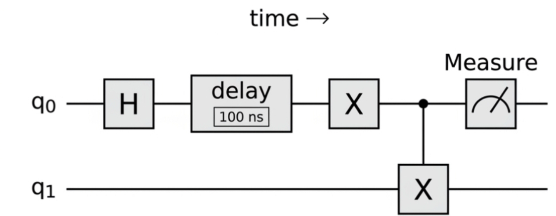
The delay instruction provides a mechanism for pausing the evolution of a qubit for a specified duration. Although the qubit is idle during this period, the instruction plays an important role in shaping how operations align across multiple qubits. Strategic delays can help mitigate crosstalk, coordinate entangling gates, or implement sequences designed to preserve coherence.


OPENQASM 3;

qubit q[1];

h q[0];
delay[200ns] q[0];
x q[0];


The delay statement pauses operations on the qubit for two hundred nanoseconds before the next gate executes. On real hardware, such pauses are sometimes necessary when coordinating operations across qubits that share control electronics or physical coupling pathways.

One of the most important applications of explicit timing appears in dynamical decoupling sequences. These sequences insert carefully spaced pulses into a circuit to counteract environmental noise. By periodically flipping the qubit state, the system averages out certain sources of decoherence that would otherwise degrade the computation.

Designing these sequences requires precise control over timing intervals. OpenQASM 3.0 allows developers to represent those intervals directly in the circuit description rather than relying entirely on compiler heuristics. This capability becomes particularly useful in experiments where maintaining coherence over long circuits is essential.

Timing instructions also improve transparency when analyzing circuit behavior. Researchers examining an OpenQASM program can immediately see how operations are scheduled relative to each other, providing insight into how the circuit interacts with the physical constraints of the device.

Timing Control and Hardware Stability

When working with real quantum processors, timing is rarely an abstract concept. Each gate corresponds to a physical interaction lasting a measurable amount of time. Superconducting qubits respond to microwave pulses with durations measured in nanoseconds, while trapped-ion systems rely on laser interactions with different temporal characteristics. Regardless of the platform, the sequence and spacing of these operations influence the stability of the experiment.

Delays inserted into a circuit can serve several purposes beyond simple synchronization. In multi-qubit systems, neighboring qubits can unintentionally influence one another through residual couplings. Carefully scheduling operations and introducing short idle periods can help reduce unwanted interference. Researchers sometimes experiment with different delay intervals to observe how qubit coherence behaves over time.

Another common application involves dynamical decoupling, a technique borrowed from nuclear magnetic resonance. The basic idea is to periodically flip the qubit state using carefully timed pulses. By doing so, environmental noise affecting the qubit can average out, extending the effective coherence time. These sequences often rely on specific patterns of delays and rotations distributed across the circuit timeline.


OPENQASM 3;

qubit q[1];

h q[0];
delay[100ns] q[0];
x q[0];
delay[100ns] q[0];
x q[0];
delay[100ns] q[0];
h q[0];


Although this simplified example illustrates the idea conceptually, real dynamical decoupling routines may contain dozens of pulses arranged with carefully calibrated intervals. OpenQASM 3.0 allows those structures to be expressed explicitly, making the timing behavior visible rather than hidden inside compiler-generated schedules.

The growing importance of timing awareness reflects a broader trend in quantum computing. As circuits become deeper and experiments grow more complex, the physical environment surrounding qubits plays an increasingly important role. Languages that allow programmers to reason about timing directly offer a more realistic view of how algorithms interact with hardware.

Technique 4: Embedded Pulse-Level Calibration

While most quantum programmers interact with gates such as X, H, or controlled operations, the hardware itself ultimately executes sequences of analog pulses. These pulses manipulate qubit states through carefully shaped microwave or laser signals. The mapping between a high-level gate and the underlying pulse sequence is typically defined through calibration routines maintained by the hardware provider.

OpenQASM 3.0 introduces a mechanism that allows pulse-level calibrations to be described directly within the language through the defcal construct. Calibration definitions connect abstract gates to the pulse instructions that implement them on a specific device. This feature enables developers to experiment with custom operations while remaining within the same circuit description environment.

A calibration block can define how a particular gate should be executed on a given qubit. In practice these definitions reference pulse primitives supported by the hardware backend. Although the exact syntax may vary depending on the control system, the conceptual structure remains consistent: associate a gate operation with a sequence of physical control signals.


OPENQASM 3;

defcal x q {
    play gaussian(160ns, 0.5) q;
}


This calibration definition associates the X gate with a Gaussian-shaped pulse lasting 160 nanoseconds. The amplitude and shape parameters determine how the pulse interacts with the qubit’s control channel. Real calibration routines often involve significantly more complex pulse shapes, including derivative removal techniques and phase adjustments designed to reduce leakage into higher energy states.

Embedding calibration definitions directly within a circuit description allows experimentalists to explore new control strategies without rewriting large portions of the software stack. Researchers developing custom gates or investigating hardware behavior can modify the pulse definition while keeping the surrounding circuit structure intact.

In many laboratory environments, calibration routines are refined continuously as devices drift or environmental conditions change. Languages capable of expressing both circuit logic and calibration behavior provide a convenient bridge between algorithm development and hardware experimentation.

OpenQASM 3.0 also allows external pulse grammars to be referenced through the defcalgrammar directive. This mechanism enables integration with specialized pulse programming environments while preserving compatibility with the broader language structure.


OPENQASM 3;

defcalgrammar "openpulse";


With this directive the circuit indicates that pulse definitions should follow a specific grammar understood by the underlying control system. Such flexibility allows OpenQASM programs to remain portable while still interacting with device-specific calibration layers.

Technique 5: Classical Control Flow Inside Quantum Programs

Quantum circuits are often introduced as fixed structures: a sequence of gates applied to qubits followed by measurement. In practice, many experimental routines require a more flexible execution model. Measurements taken during a computation can reveal information that must influence later steps. Earlier quantum assembly languages provided only limited support for this interaction between quantum measurements and classical decision-making.

OpenQASM 3.0 expands the role of classical logic within quantum programs. The language introduces constructs familiar from conventional programming environments, including variables, loops, conditional branching, and reusable subroutines. These additions allow a circuit description to contain both quantum operations and the classical logic that determines how those operations unfold.

Consider a scenario in which a quantum experiment must repeat an operation until a particular measurement outcome is obtained. Instead of constructing multiple separate circuits, a programmer can embed a loop directly within the OpenQASM program. The measurement result can be stored in a classical variable and evaluated to determine whether the process should continue.


OPENQASM 3;

qubit q[1];
bit result;

result = 0;

while (result == 0) {
    h q[0];
    measure q[0] -> result;
}


In this example the program repeatedly prepares a qubit in superposition and measures it until the classical variable records a value of one. Although the circuit is simple, the structure illustrates how classical feedback can influence the flow of execution. The quantum operations remain embedded within a broader program that reacts to measurement results.

OpenQASM also allows developers to define reusable subroutines. Subroutines help organize larger circuits into logical components, making complex programs easier to maintain and analyze. Instead of repeating sequences of gates throughout a circuit, the programmer defines a reusable block that can be invoked whenever needed.


OPENQASM 3;

def entangle(qubit a, qubit b) {
    h a;
    cx a, b;
}

qubit q[2];

entangle(q[0], q[1]);


This structure resembles a function definition in classical programming languages. The subroutine defines a reusable entangling operation that can be applied to any pair of qubits passed as arguments. As circuits expand toward dozens or hundreds of qubits, such modular structures become increasingly valuable.

These classical control constructs also play an important role in hybrid quantum algorithms. Variational algorithms such as the Variational Quantum Eigensolver or the Quantum Approximate Optimization Algorithm repeatedly adjust circuit parameters based on classical optimization routines. Although the optimization itself typically runs outside the quantum program, OpenQASM’s control features make it easier to represent parameterized circuit structures and iterative procedures.

Technique 6: Register Aliasing and Advanced Qubit Management

As quantum processors scale beyond a handful of qubits, circuit organization becomes a practical challenge. Managing large collections of qubits often requires dividing registers into logical groups that correspond to different roles within the computation. Some qubits may store data, others may serve as ancilla qubits for intermediate calculations, and still others may function as measurement registers.

OpenQASM 3.0 introduces mechanisms that simplify this management through register slicing and aliasing. Instead of treating every qubit as an isolated element, developers can reference subsets of larger registers and combine them into new logical structures. This capability becomes particularly helpful when building modular circuit components.

Register slicing allows a portion of a register to be referenced without redefining the qubits individually. The notation resembles slicing operations in classical programming languages.


OPENQASM 3;

qubit q[6];

qubit data[3] = q[0:3];
qubit ancilla[3] = q[3:6];


In this example the original register containing six qubits is divided into two logical groups. The first three qubits become the data register, while the remaining three serve as ancilla qubits. Operations can then be applied to each group independently without losing the connection to the original register structure.

Aliasing provides a related capability by allowing new names to refer to existing qubit resources. This can simplify circuit descriptions when certain qubits must participate in multiple logical roles throughout different stages of a computation.

These organizational tools become increasingly valuable when designing circuits for processors containing dozens or even hundreds of qubits. Without structured register management, large circuits quickly become difficult to interpret. By grouping qubits logically, OpenQASM programs can remain readable even as their scale increases.

Effective qubit organization also supports collaboration among researchers. When circuits are shared across teams or institutions, clear register structures help communicate the intended role of each qubit within the algorithm. The language therefore contributes not only to execution but also to the clarity of the circuit’s conceptual design.

Technique 7: Parameterized Circuits and Hybrid Workflows

Many of the most promising quantum algorithms today rely on hybrid workflows where quantum circuits interact closely with classical optimization routines. Instead of running a circuit once with fixed parameters, these algorithms repeatedly execute parameterized circuits while classical software updates those parameters in search of better results. This interaction lies at the core of methods such as the Variational Quantum Eigensolver and the Quantum Approximate Optimization Algorithm.

OpenQASM 3.0 introduces mechanisms for defining circuit parameters through input and output modifiers. These constructs allow a circuit to receive parameters from an external program and return measurement results that can guide further computation. In effect, the circuit becomes part of a larger feedback loop connecting quantum hardware with classical optimization software.


OPENQASM 3;

input float theta;

qubit q[1];

rx(theta) q[0];
measure q[0];


In this example the parameter theta is provided externally when the circuit executes. Classical software can adjust the value of this parameter repeatedly while observing how the measurement results change. The process allows a hybrid algorithm to explore different circuit configurations while relying on the quantum device to evaluate the resulting quantum states.

Parameterized circuits are especially valuable in the NISQ era where quantum processors remain limited in scale and coherence. Instead of constructing extremely deep circuits that attempt to solve problems directly, hybrid algorithms combine shorter quantum circuits with classical optimization strategies. OpenQASM’s parameter interface provides a convenient bridge between these two domains.

Best Practices for Professional Circuit Design in OpenQASM 3.0

Writing effective quantum circuits requires more than syntactic familiarity with the language. As circuits grow in complexity, careful design decisions determine whether a program remains understandable and efficient. Several practices have emerged among researchers working directly with OpenQASM-level circuit descriptions.

Modularity is one of the most valuable principles. Breaking large circuits into smaller subroutines makes it easier to test individual components and reuse them across experiments. Subroutines also help communicate the intent behind specific operations, allowing collaborators to understand the structure of a circuit more quickly.

Another important consideration involves circuit depth. Because qubits remain fragile physical systems, every additional gate introduces potential noise. Using gate modifiers and carefully structured operations can often reduce the number of instructions required to implement a transformation. Even small reductions in circuit depth can noticeably improve experimental results.

Debugging quantum circuits often requires examining both simulation results and hardware executions. Simulators provide an idealized environment where the mathematical behavior of the circuit can be verified. Running the same circuit on hardware reveals how noise, calibration drift, and device-specific characteristics influence the outcome. Comparing the two helps identify whether unexpected behavior arises from algorithm design or hardware limitations.

Another practical technique involves exporting circuits between frameworks and OpenQASM representations. Inspecting the OpenQASM output of a high-level circuit can reveal hidden assumptions about gate decompositions or scheduling decisions. This round-trip inspection process often helps researchers refine their circuits before deploying them on hardware.

Real-World Circuit Development

In experimental environments OpenQASM often serves as the layer where algorithm design meets hardware control. Researchers developing new quantum routines frequently begin with a conceptual circuit diagram, translate that structure into a framework such as Qiskit, and then examine the resulting OpenQASM representation to understand how the instructions will actually execute.

Consider a scenario involving an adaptive measurement protocol. A circuit might prepare an entangled state, measure one qubit, and then apply corrective operations to another qubit depending on the measurement outcome. The resulting OpenQASM program combines entangling gates, measurement instructions, classical conditions, and possibly timing adjustments to maintain coherence across the system.

The ability to represent all of these elements within a single language environment simplifies the experimental workflow. Instead of switching between separate tools for pulse programming, circuit construction, and classical control logic, developers can express the entire structure of the experiment in one coherent program description.

As quantum processors continue to scale, the role of such assembly-level languages is likely to grow. Higher-level frameworks will remain essential for algorithm development, but understanding how those frameworks translate into executable instructions will remain an important skill for researchers working close to the hardware.

Conclusion

OpenQASM 3.0 reflects an evolution in how quantum programs are written and executed. Earlier circuit descriptions emphasized static sequences of operations, but modern quantum experiments increasingly require dynamic behavior, classical feedback, precise timing control, and flexible parameter interfaces. The language evolved accordingly, introducing constructs that make it possible to describe these interactions directly within the circuit program.

The techniques explored here reveal how OpenQASM can function not merely as an interchange format but as a powerful environment for circuit engineering. Dynamic circuits enable adaptive algorithms, gate modifiers simplify complex operations, timing instructions expose the physical structure of experiments, calibration definitions bridge the gap between gates and pulses, classical control constructs support hybrid workflows, and register management tools make large-scale circuits easier to organize.

For researchers and developers working close to quantum hardware, understanding these capabilities provides valuable insight into how quantum computations are actually executed. As quantum systems continue to mature, assembly-level awareness will remain an important part of building reliable and efficient quantum software.

Working with OpenQASM 3.0 at this level exposes the layer where algorithm design, hardware constraints, and control systems intersect within the quantum computing stack. Mastery of these techniques does not replace high-level frameworks, but it offers a clearer understanding of the mechanisms that ultimately bring quantum circuits to life.

References

- Preskill, John. “Quantum Computing in the NISQ Era and Beyond.” Quantum 2 (2018): 79.
https://doi.org/10.22331/q-2018-08-06-79
↩ - Cross, Andrew W., Lev S. Bishop, Sarah Sheldon, Paul D. Nation, and Jay M. Gambetta.
“OpenQASM 3: A Broader and Deeper Quantum Assembly Language.”
arXiv (2021).
https://arxiv.org/abs/2104.14722
↩ - IBM Quantum Documentation. “Introduction to OpenQASM.”
https://quantum.cloud.ibm.com/docs/guides/introduction-to-qasm
↩ - OpenQASM Live Specification.
https://openqasm.com/
- Amazon Web Services. “OpenQASM in Amazon Braket.”
https://docs.aws.amazon.com/braket/latest/developerguide/braket-openqasm.html
- IBM Quantum Documentation. “Interoperability Between Qiskit and OpenQASM 3.”
https://quantum.cloud.ibm.com/docs/guides/interoperate-qiskit-qasm3
- Association for Computing Machinery (ACM).
“OpenQASM Architecture.”
https://dl.acm.org/doi/10.1145/3505636